Wannierization works best when symmetry is turned off (helps with the gauge smoothness).
NSCF INCAR updates
Parameter
Value
Reason
ISYM
-1
Symmetry might introduce extra gauge discontinuities
ALGO
Normal
LWAVE
TRUE
Basis for Wannierizaton, will need to diagonalize $\hat{H}_{\rm KS}$ again
LOCPROJ INCAR updates
Parameter
Value
Reason
LOCPROJ
“1 2 : s s p d : Hy”
Whichever projections we want to build orbitals from, see below for an explanation
NUM_WANN
IGNORED
NUM_WANN is determined by the number of projectors in LOCPROJ
ALGO
Eigenval or None
We just need to recalculate the energies or post-process using the current orbitals
SCDM INCAR updates
Parameter
Value
Reason
LSCDM
TRUE
Turns on SCDM
LWANNIER90
TRUE
Turns on Wannier90
LWRITE_MMN_AMN
TRUE
Writes .mmn and .amn files for wannier90.x inputs
ALGO
Eigenval or None
We just need to recalculate the energies or post-process using the current orbitals
CUTOFF_MU
23.0
SCDM cutoff position, value specific to this example (but can be automated). NOT w.r.t. Fermi energy
CUTOFF_SIGMA
0.5
SCDM cuttoff width
NUM_WANN
20
Number of Wannier functions (or bands)
The wannier90.amn and wannier90.mmn files contain the matrices $A_{mn}=\langle \psi_{n}| g_m\rangle $ and $M_{mn}=\langle \psi_{n}| \psi_{m}\rangle$ respectively. They are used as inputs for the MLWF procedure. The functions $g_m$ are initial projections in the LOCPROJ tag, or the SCDM orbitals.
Note that for SCDM, we are not bound by NUM_WANN, but for LOCPROJ we are bound by how many projectors we choose (e.g. a set of $s$ and $p$ orbitals have $1+3$ total bands in a non-spin polarized calculation).
For this examle, we choose $s$, $s$, $p$, $d$ to sum to 10 bands per element ($1+1+3+5$).
[!WARNING ]""
The LOCPROJ tag requires a multiline string, which current pymatgen cannot work with. For this reason, you must open the INCAR file in the directory and append the following
! NbTi/locproj/INCAR
! ...
LOCPROJ="1 2 : s s p d : Hy"
The local orbitals are defined as sites : angular character : radial character, and so 1 2 : s s p d: Hy means “project onto two sets of $s$, one set of $p$ and $d$ Hydrogenic orbitals for both elements in sites 1 and 2 of the POSCAR”.
The multiple specifications in LOCPROJ requires a semicolon or a multiline string, which will cause problems anytime Custodian or pymatgen wants to edit/pase the INCAR file. This may result in a failed vasprun.xml.
The VASP section on LOCPROJ has more information about the types of orbital projections one can use.
Alternatively, for projections one can create a wannier90.win file beforehand with a projections block (similar to Q.E.)
However, I would not recommend this as VASP does not support hybrid projections in this format (e.g. the $sp-2$ projection will work when specified through LOCPROJ = 1 : sp-2 : Hy, but not through the wannier90.win file!)
Interpolating with Wannier90
Insert the following in the wannier90.win file that was created automatically by VASP. We will use the default gauge (i.e. no MLWF optimization)
! locproj/wannier90.win & scdm/wannier90.win &
num_iter=0! Don't optimize the spread
dis_num_iter=0! Don't do any disentanglement
write_hr=.true.! writes TB hamiltonian data
write_xyz=.true.! writes atomic positions and Wannier centres in cartesian coordinates
bands_plot=.true.bands_num_points=200! kpath must match the one by VASP
beginkpoint_pathG0.00.00.0X0.00.50.0X0.00.50.0M0.50.50.0M0.50.50.0G0.00.00.0G0.00.00.0Z0.00.00.5Z0.00.00.5R0.00.50.5R0.00.50.5A0.50.50.5A0.50.50.5Z0.00.00.5R0.00.50.5X0.00.50.0M0.50.50.0A0.50.50.5endkpoint_path! This part was generated automatically by VASP
num_bands=42num_wann=20...
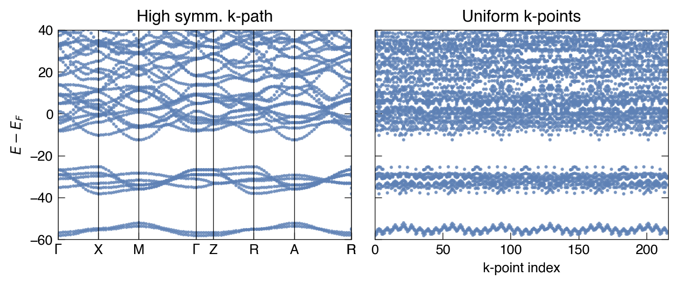
fig, ax = plt.subplots(2,1, dpi =200, figsize=(4.0, 6), sharey=True)
make_pretty(fig,ax)
ax[0].plot(bs.distance, bs.bands[Spin.up].T - nscf.efermi, '.', color ='C0', alpha=0.7, ms=3)
# ax[0].plot(scdm_kpts, scdm_energies.T - nscf.efermi, '-', color = 'k', lw = 1.5)# ax[0].axhline(scdm_incar['CUTOFF_MU'] - nscf.efermi, ls='-.', color = 'r', lw = 2.0)ax[0].set_xticks(scdm_ticks.dist)
ax[0].set_xticklabels(scdm_ticks.label)
[ax[0].axvline(x, lw=0.5, c='k') for x in scdm_ticks.dist]
ax[0].set_title("High symm. k-path")
ax[0].set_ylim(-60,40)
ax[0].set_xlim(scdm_ticks.dist.iloc[0], scdm_ticks.dist.iloc[-4])
ax[0].set_ylabel(r"$E-E_F$")
ax[1].plot(nscf.get_band_structure().bands[Spin.up].T - nscf.efermi, '.', color ='C0', alpha=0.7, ms=3)
ax[1].set_xlabel("k-point index")
ax[1].set_xlim(0, nscf.get_band_structure().bands[Spin.up].shape[1])
ax[1].set_title("Uniform k-points")
# ax[1].plot(locproj_kpts, locproj_energies.T - nscf.efermi, '-', color = 'k', lw = 1.5)# ax[1].set_xticks(scdm_ticks.dist)# ax[1].set_xticklabels(scdm_ticks.label)# [ax[1].axvline(x, lw=0.5, c='k') for x in scdm_ticks.dist]# ax[1].set_title("LOCPROJ")# ax[1].set_ylim(-60,40)# ax[1].set_xlim(scdm_ticks.dist.iloc[0], scdm_ticks.dist.iloc[-4])plt.tight_layout()
plt.show()
nscf.get_band_structure().bands[Spin.up].shape[1]
216
Show code
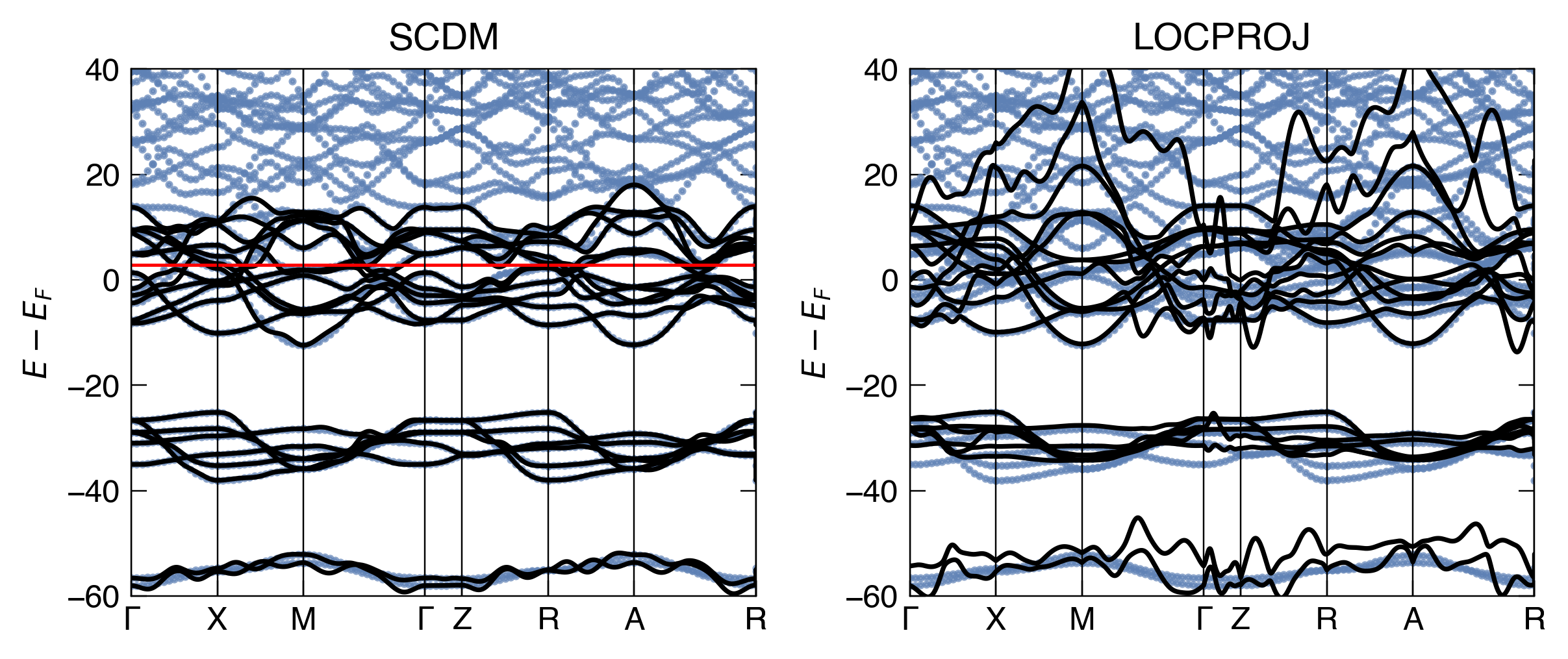
fig, ax = plt.subplots(2,1, dpi =350, figsize=(5,8), sharex=True)
make_pretty(fig,ax)
ax[0].plot(bs.distance, bs.bands[Spin.up].T - nscf.efermi, '.', color ='C0', alpha=0.7, ms=3)
ax[0].plot(scdm_kpts, scdm_energies.T - nscf.efermi, '-', color ='k', lw =1.5)
ax[0].axhline(scdm_incar['CUTOFF_MU'] - nscf.efermi, ls='-', color ='r', lw =1.0)
ax[0].set_xticks(scdm_ticks.dist)
ax[0].set_xticklabels(scdm_ticks.label)
[ax[0].axvline(x, lw=0.5, c='k') for x in scdm_ticks.dist]
ax[0].set_title("SCDM")
ax[0].set_ylim(-60,40)
ax[0].set_xlim(scdm_ticks.dist.iloc[0], scdm_ticks.dist.iloc[-4])
ax[0].set_ylabel(r"$E-E_F$")
ax[1].plot(bs.distance, bs.bands[Spin.up].T - nscf.efermi, '.', color ='C0', alpha=0.7, ms=3)
ax[1].plot(locproj_kpts, locproj_energies.T - nscf.efermi, '-', color ='k', lw =1.5)
ax[1].set_xticks(scdm_ticks.dist)
ax[1].set_xticklabels(scdm_ticks.label)
[ax[1].axvline(x, lw=0.5, c='k') for x in scdm_ticks.dist]
ax[1].set_title("LOCPROJ")
ax[1].set_ylim(-60,40)
ax[1].set_ylabel(r"$E-E_F$")
ax[1].set_xlim(scdm_ticks.dist.iloc[0], scdm_ticks.dist.iloc[-4])
plt.tight_layout()
plt.show()
Note that SCDM gets a much better band-structure without any optimization (although we provided disentanglement options, whereas with LOCPROJ we did not disentangle, so not really an apples to apples comparison).
MLWF
The VASP2WANNIER90 can insert more information into the wannier90.win file through the WANNIER90_WIN tag. However, doing so requires multiline strings, which are not handled well by pymatgen (yet).
If we need to modify the Wannierization process, we must remove the wannier90.win file before running VASP or else VASP will read this file and use the settings written in this file (e.g. when increasing k-points in the NSCF calculation, not removing the previous wannier90.win file will result in an error.)
I detail here the parameters for MLWF generation through wannier90.x.
In WANNIER90_WIN tag or wannier90.win file
LOCPROJ
Parameter
Value
Reason
num_iter
1000
Iterations for spread optimization
dis_num_iter
500
Need to optimize subspace before spread optimization (disentanglement)
dis_froz_min
0 (eV)
Minimum of disentanglement window
dis_froz_max
30 (eV)
Top of disentanglement window
SCDM
Parameter
Value
Reason
num_iter
1000
Iterations for spread optimization
dis_num_iter
0
Subspace is already disentangled, disentangling again can worsen the quality of the WFs
Disentanglement and energy windows are not shifted to the Fermi energy.
Excluding bands
Usually, we are not interested in semi-core states, such as the ones below -50 eV. There is no tag in the INCAR for this, it is a parameter in the *.win file.
Unfortunately, for VASP<6.5.0 versions, the interface will not take into account the exclude_bands tag.
In the above example we have 2 semi-core states ($s$ orbitals) and six valence states ($p$ orbitals), so we exclude states 1-6 from the MLWF process.
In INCAR:
Parameter
Value
Reason
WANNIER90_WIN
“exclude_bands = 6”
String that gets inserted in wannier90.win, how many bands to exclude from the overlap matrices
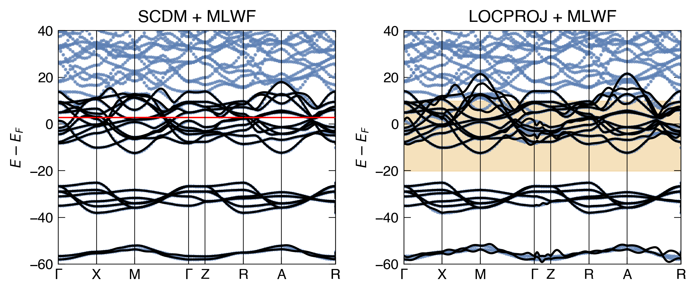
fig, ax = plt.subplots(2,1, dpi =350, figsize=(5,8), sharex=True)
make_pretty(fig,ax)
ax[0].plot(bs.distance, bs.bands[Spin.up].T - nscf.efermi, '.', color ='C0', alpha=0.7, ms=3)
ax[0].plot(scdm_mlwf_kpts, scdm_mlwf.T - nscf.efermi, '-', color ='k', lw =1.5)
ax[0].axhline(scdm_incar['CUTOFF_MU'] - nscf.efermi, ls='-', color ='r', lw =1)
ax[0].set_ylabel(r"$E-E_F$")
ax[1].plot(bs.distance, bs.bands[Spin.up].T - nscf.efermi, '.', color ='C0', alpha=0.7, ms=3)
ax[1].plot(locproj_mlwf_kpts, locproj_mlwf.T - nscf.efermi, '-', color ='k', lw =1.5)
ax[1].fill_between(np.linspace(0,scdm_mlwf_kpts[-1],100), dis_froz_min - nscf.efermi, dis_froz_max - nscf.efermi, alpha=0.3, color='C1', label ="Frozen window")
ax[1].set_ylim(-60,40)
[ax[0].axvline(x, lw=0.5, c='k') for x in scdm_ticks.dist]
ax[0].set_title("SCDM + MLWF" )
[ax[1].axvline(x, lw=0.5, c='k') for x in scdm_ticks.dist]
ax[1].set_title("LOCPROJ + MLWF" )
ax[1].set_ylabel(r"$E-E_F$")
# limitsax[1].set_xticks(scdm_ticks.dist)
ax[1].set_xticklabels(scdm_ticks.label)
ax[1].set_xlim(scdm_ticks.dist.iloc[0], scdm_ticks.dist.iloc[-4])
ax[0].set_ylim(-60,40)
# ax[1].legend(loc="upper right")plt.tight_layout()
plt.show()
Show code
fromatomate2_wannierimport get_omega
frompathlibimport Path
SCDM_MLWF_PATH ="./scdm_mlwf"LOCPROJ_MLWF_PATH ="./locproj_mlwf"scdm_omega = {s: get_omega(Path(SCDM_MLWF_PATH, "wannier90.wout")) for s in Spin}
proj_omega = {s: get_omega(Path(LOCPROJ_MLWF_PATH, "wannier90.wout")) for s in Spin}
# proj_omega = {s: get_omega(Path(dir, "proj", f"{elname}_{s.name}.wout")) for s in Spin}fig, ax = plt.subplots(dpi =250 , figsize=(4,2.4))
(fig, ax)
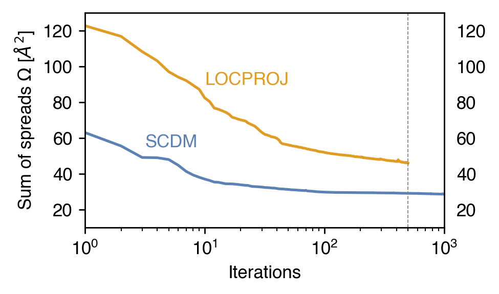
ax.plot(scdm_omega[Spin.up][:,-1], '-C0', label="SCDM")
# ax.plot(scdm_omega[Spin.down][:,-1], '-', label="PD+SCDM")ax.plot(proj_omega[Spin.up][:,-1], '-C1', label="LOCPROJ")
ax.text(10**1, 90, "LOCPROJ", c="C1")
ax.text(10**.5, 55, "SCDM", c="C0")
xticks = [10^j for j inrange(3)]
ax.axvline(500, lw=0.5, color='gray', ls="--")
ax.set_xticks(xticks)
# ax.plot(proj_omega[Spin.up][:,-1], '-C3', label="ED+AO")ax.tick_params(axis='y', which='both', labelleft=True, labelright=True)
ax.set_ylabel(r"Sum of spreads $\Omega$ [$\AA^2$]")
ax.set_xlabel(r"Iterations")
ax.set_xscale('log')
ax.set_xlim(1, 1e3)
ax.set_ylim(10, 130)
# ax.legend()plt.tight_layout()
plt.show()
It seems the spread minimization of the LOCPROJ run did not reach finish optimizing, it would be best to increase the number of iterations.
fromatomate2_wannier.utilitiesimport parse_xyz
distances = []
for folder in [SCDM_MLWF_PATH, LOCPROJ_MLWF_PATH]:
closest = []
vasprun = Vasprun(Path(LOCPROJ_MLWF_PATH, "vasprun.xml"))
wann_centres = parse_xyz(Path(folder, "wannier90_centres.xyz"))[0]
sites = vasprun.final_structure.sites
dist_to_atom = {site.label: [] for site in sites}
struct = vasprun.final_structure
fracs = struct.lattice.get_fractional_coords(wann_centres)
dist_array = []
for (i,x0) inenumerate(fracs):
dist = {}
for site in struct.sites:
d, _ = site.lattice.get_distance_and_image(x0, site.frac_coords)
dist[site] = d
# get site with smallest distance to wannier center closest_site =min(dist, key=dist.get)
# distances.append({closest_site: dist[closest_site]}) dist_array.append({closest_site.label: dist[closest_site]})
dist_to_atom[closest_site.label].append(dist[closest_site])
distances.append(dist_array)
Sanitized LOCPROJ: []
Sanitized LOCPROJ: []


/Users/ar/venvs/atomate2/lib/python3.12/site-packages/pymatgen/io/vasp/outputs.py:1353: UserWarning: No POTCAR file with matching TITEL fields was found in

  if potcar := self.get_potcars(path):
/Users/ar/venvs/atomate2/lib/python3.12/site-packages/pymatgen/io/vasp/outputs.py:1364: UserWarning: No POTCAR file with matching TITEL fields was found in

  potcar = self.get_potcars(path)
Atomic centered WFs
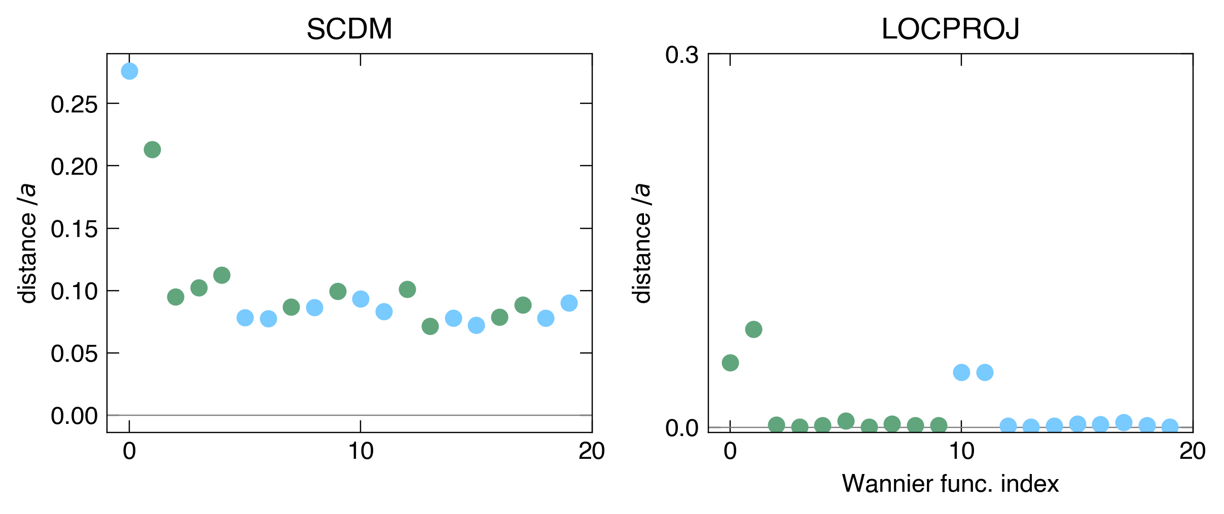
Even though SCDM has a great spread and can be very automatic compared to the LOCPROJ method, it fails in both symmetry and selective-localization. In other words, the orbitals generated will most definitely be far away from the atomic positions, and thus will not be very useful for tasks that require assigning wavefunctions to atoms (like estimating exchange interactions in TB2J).
Show code
fig, ax = plt.subplots(2,1, dpi =350, figsize=(5,8), sharex=True)
make_pretty(fig,ax)
ax[0].axhline(0, lw=0.5, color="gray")
ax[1].axhline(0, lw=0.5, color="gray")
bins = np.linspace(0,4,10)
color_dict = {"Nb": "#61A57D", "Ti": "#78caff"}
lattice_const = struct.lattice.c
data = np.array([[[ val / c, color_dict[key]] for key,val in d.items()] for d in distances[0]], dtype=np.object_).squeeze()
[ax[0].plot(i, v[0], c=v[1], marker='o') for i,v inenumerate(data)]
data = np.array([[[ val / c, color_dict[key]] for key,val in d.items()] for d in distances[1]], dtype=np.object_).squeeze()
[ax[1].plot(i, v[0], c=v[1], marker='o') for i,v inenumerate(data)]
ax[1].set_xlabel("Wannier func. index")
# ax[1].set_xticks(range(0,21,5))ax[1].set_ylabel(r"distance $ / a$")
ax[0].set_ylabel(r"distance $ / a$")
# ax[1].set_yticks([0,1])ax[0].set_title("SCDM")
ax[1].set_title("LOCPROJ")
ax[1].set_yticks([0, 0.3])
ax[1].set_xticks(range(0,21, 10))
plt.tight_layout()
plt.show()
Interpolating the Hamiltonian ourselves (optional)
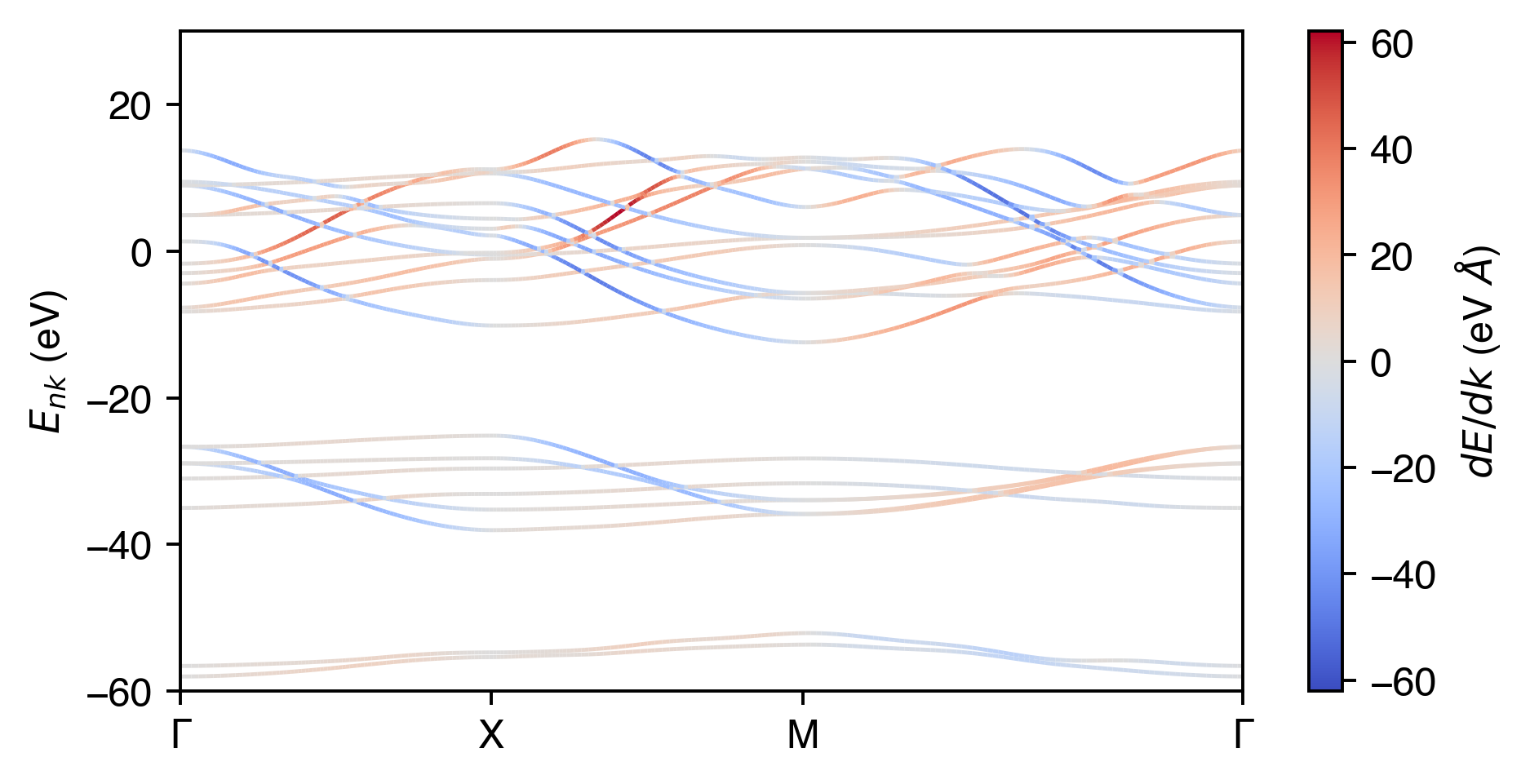
Wannier90 can interpolate the Hamiltonian in a path defined under kpoint_path. However, editing this file can become tedious. If we set write_hr and write_xyz to .true. in the wannier90.win file, then Wannier90 will write the Wannier Hamiltonian elements $\langle m\mathbf{0}| H |n\mathbf{R}\rangle$ and the cartesian lattice indices $\mathbf{R}$ needed to pefrorm the interpolation
$$
H_{mn}^W=\sum_{\mathbf{R}}e^{i\mathbf{k}\cdot\mathbf{R}}\langle m\mathbf{0}| H |n\mathbf{R}\rangle
$$
We will perform an interpolation through $\Gamma \rightarrow X\rightarrow M \rightarrow \Gamma$
kp_sym = \
np.array([
[0.0, 0.0, 0.0], # G [0.0, 0.5, 0.0], # X [0.5, 0.5, 0.0], # M [0.0, 0.0, 0.0], # G ])
num_sym = kp_sym.shape[0]
nk_tot =2**8kpath_to_interpolate = np.vstack([np.linspace(kp_sym[j], kp_sym[j+1], nk_tot // (num_sym -1), endpoint=False) for j inrange(num_sym -1)])
k_distance = np.cumsum(np.linalg.norm(np.vstack([[0,0,0], np.diff(kpath_to_interpolate, axis=0)]), axis=1))
fromTB2J.wannierimport parse_atoms, parse_ham, parse_xyz
importscipyasspimportgcnum_wann, hr, rvecs = parse_ham("./scdm_mlwf/wannier90_hr.dat")
xcart = parse_xyz("./scdm_mlwf/wannier90_centres.xyz")
atoms = parse_atoms("./scdm_mlwf/wannier90.win")
degen = rvecs.astype(float)
H_mnR_frac = {}
for R_frac, H in hr.items():
# R_frac is a tuple (i, j, k) in fractional coordinates H_mnR_frac[R_frac] = H # Key is (i, j, k) fractionalR_vecs = np.array(list(H_mnR_frac.keys())) # fractional coordinatesH_vals = np.array(list(H_mnR_frac.values()))
H_vals_w = H_vals / degen[:, None, None] # unfold crystal symmetryphases = np.exp(2j * np.pi * kpath_to_interpolate @ R_vecs.T)
H_mnK = (phases[:, :, None, None] * H_vals_w[None, :, :, :]).sum(axis=1)
H_mnK =2*H_mnK # idk why we need twice its value to match dft, maybe a cartesian / fractional convention# get eigenvaluesE_nk, U_mnk = sp.linalg.eigh(H_mnK)
gc.collect() # check if we can release some memory
59014
Calculating Bloch velocity
Show code
frommatplotlib.collectionsimport LineCollection
fig, ax = plt.subplots(dpi=350, figsize=(6,3))
band_velocities = np.array([np.gradient(band, k_distance) for band in E_nk.T])
vmin = np.min(band_velocities)
vmax = np.max(band_velocities)
vval = np.max([np.abs(vmin), vmax])
norm = plt.Normalize(vmin=-vval, vmax=vval)
for band, scalar_velocity inzip(E_nk.T, band_velocities):
points = np.array([k_distance / k_distance[-1], band - nscf.efermi]).T.reshape(-1, 1, 2)
segments = np.concatenate([points[:-1], points[1:]], axis=1)
# Pass the norm object to LineCollection lc = LineCollection(segments, cmap='coolwarm', norm=norm, lw=1)
# Set the values used for colormapping lc.set_array(scalar_velocity)
ax.add_collection(lc)
ax.set_xticks(scdm_ticks.dist / scdm_ticks.dist.iloc[3])
ax.set_xticklabels(scdm_ticks.label)
ax.set_xlim(0, 1)
ax.set_ylim(-60, 30)
ax.set_ylabel(r"$E_{nk}$ (eV)")
cbar = fig.colorbar(lc, ax=ax, label=r'$dE/dk$ (eV $\AA$)')
plt.show()