Transverse Ising model
Transfer matrix methods
WORK IN PROGRESS (I believe plots are wrong)
Previously I showed a certain type of Ising model called the potts model. However, in such simulations we only performed a state-space evolution, so called a thermalization (from an initial configuration).
In a quantum system, there can be fluctuations in time as well, and thus we need for a Path-integral method of simulation.
Quantum Monte Carlo
We can emply the Wolff algorithm to accelerate the flipping of spins by instead flipping a cluster of spins. In this algorithm (there are other cluster algorithms), a randomly selected spin (uniform sampling) is connected to its neighbours iff they share the same sign. The probability that both neighbors have the same sign is \(1-e^{-2\beta J}\), and is used for calculating adding links to the cluster (since they are assumed frozen). E.g. if \(s_{j_0}=s_{j_0+1}\), then \(s_{j_0+1}\) is added to the cluster if rand() < 1-exp(-2*β*J)
Trotterization
Furthermore, since spins can flip as a function of (imaginary) time, they also need to be added
This is easily seen from the trotterization of the Hamiltonian,
\[ \begin{aligned} H&=-J\sum_{i}\sigma^z_{i}\sigma^z_{i+1}-h\sum_{i}\sigma_i^x\\ &=H_z+H_x, \end{aligned} \]
and then the partition function
\[ \begin{aligned} Z&=\mathrm{Tr}\;e^{-\beta H},\\ &= \mathrm{Tr}\;e^{-\beta(H_z+H_x)},\\ &=\lim_{M\rightarrow \infty}\qty(e^{\beta H_z/M}e^{\beta H_x/M})^M,\\ \end{aligned} \]
where \(\beta=\Delta \tau M\) evolves in imaginary time.
This is the result of Path-Integral QMC: the 1D quantum Ising model is mapped to a 2D classical Ising model.
\[ S=-K_s\sum_{i,n}\sigma_{i,n}\sigma_{i+1, n}-K_t \]
This allows for more statistically independent configurations (because of detailed balance?) to be generated in fewer step, compared to single spin-flip methods.
The magnetization \(|m|\) can distinguish between a ferromagnetic (FM) and a paramagnetic 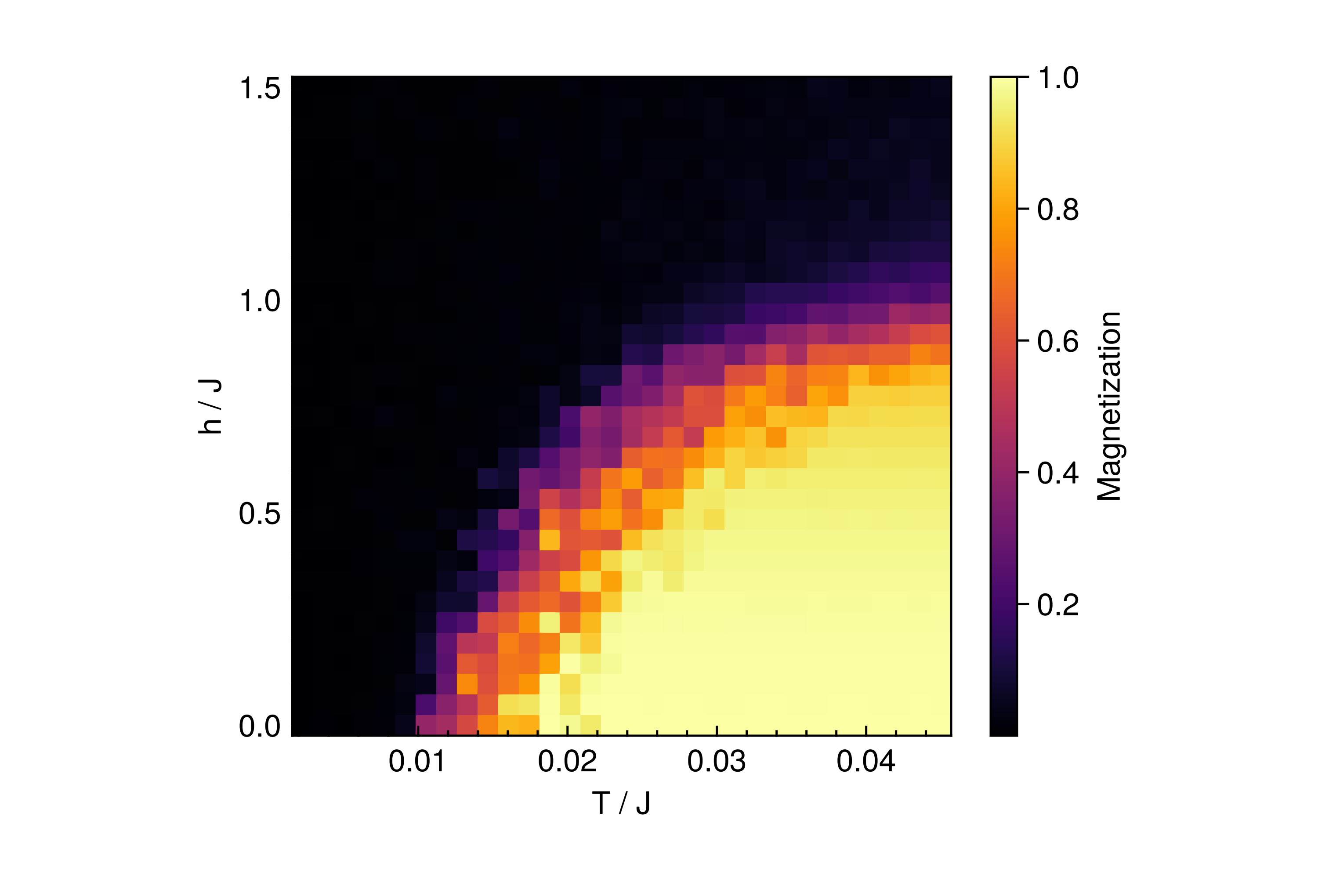
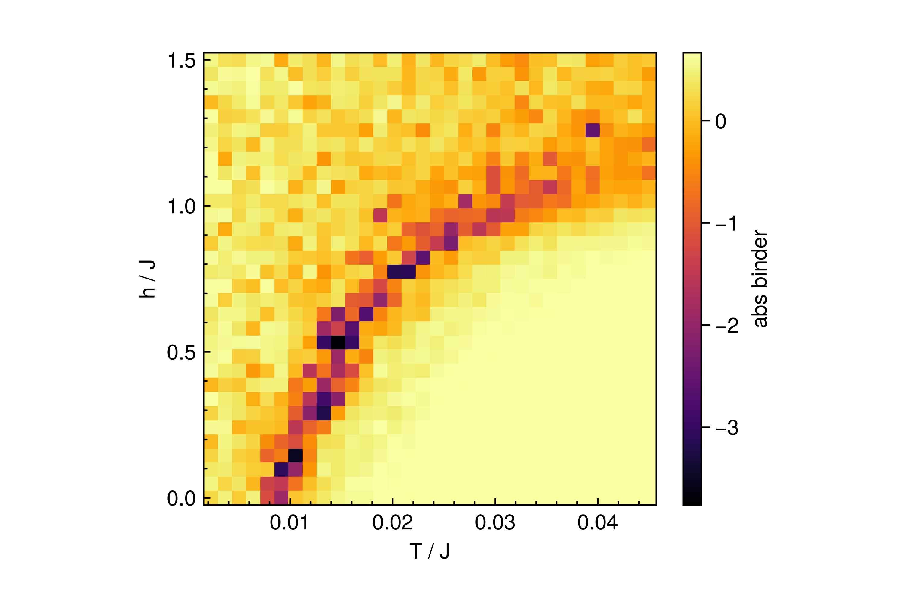
THe Binder cumulant is defined as \[ U_L=1-\frac{\expval{m^4}}{3\expval{m^2}^2} \]